The True Nature of Accelerating Objects, in Code - Part II.
(If you missed part 1 of this discussion, the following won’t make a ton of sense. Read Part 1 here.)
Recap: we’ve used a seemingly valid way to change the position and velocity of a moving particle. However, upon closer inspection, it turned out to not give physically realistic motion.
Here’s a table of data showing successive positions for an object undergoing accelerative motion. The first column has the time (in seconds). The second column calculates the position using standard kinematics. The third column uses the not quite right code from the previous post.
| t | position (good) | position (bad) |
|---|---|---|
| 0 | 0 | 0 |
| 1 | 0.5 | 1 |
| 2 | 2.0 | 3 |
| 3 | 4.5 | 6 |
| 4 | 8.0 | 10 |
| 5 | 12.5 | 15 |
Clearly there is a discrepancy. (The series of numbers in the bad column is not worthless though. It generates triangular numbers which have many interesting properties.)
Alright. We’ve got our problem. Now let’s solve it. We need to translate our equation of motion for an object undergoing uniform acceleration into a set of javascript instructions.
\[x(t) = x_0 + v_0t + \frac{1}{2} a t^2 \;\; \Rightarrow \;\; \textrm{CODE}\]We learned in Part 1 that we can’t just plop this equation in and be done - instead, we need to iteratively add changes in velocity to an already moving particle.
Now, the basic strategy we employed in the previous example will be fine, we just need to tweak how we modify the position value.
To understand what we need to do, let’s take a look at the calculus of kinematics.
Velocity is defined as the derivative of position with respect to time:
\[v = \frac{dx}{dt}\]Using the fundamental theorem of calculus, we can say that position is given by the following integral:
\[x = \int v\; dt\](we’re leaving out a constant - it’s ok if we say the motion starts from $x = 0$)
Now, if $v$ doesn’t change in time, then we can remove it from inside the integral and we end up with
\[x = v \int dt = v t\]Easy peasy lemon squeezy. However, when the velocity is changing, then we can’t take it out of the integral. We actually have to do the integral. Any integral, if you recall, is just the area under the curve:
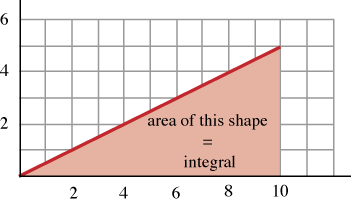
In this image, it would just be the area of that triangle, which is of course half the base times the height:
\[\textrm{area of triangle}\; = \frac{1}{2} \times 10 \times 5 = 25\]Now, let’s draw a graph that shows the velocity as a function of time. Time is on the horizontal axis, velocity on the vertical. Essentially, it’s a plot of:
\[v = a t\]where $a$ is the acceleration (or rate of change of the velocity). It’s also the slope of the green line.
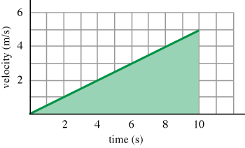
We see the object starts from rest, then increases speed in a linear fashion. To find the distance traveled during this time, we just need to find the area underneath the green line, as we did above. This of course is just the triangle again. The only difference this time is that the units of the axes are different. On the bottom is time measured in seconds, on the vertical is velocity measured in meters per second. But the basic idea is the same:
\[x = \int v\; dt = \frac{1}{2} \times 10 \;\textrm{s}\; \times 5 \; \textrm{m/s} = 25 \; \textrm{m}\]Let’s look at this equation in more detail. The $\frac{1}{2}$ and the $5 \; \textrm{m/s}$ can be interpreted as the calculation of the average velocity. The average velocity, $\bar{v}$ between any two times for this graph would be given by:
\[\bar{v} = \frac{v_1 + v_2}{2}\]If the first time is zero, when the object is at rest, then $v_1 = v_{\left(t=0 \right)} = 0$ and if the final time is at the end of the graph, $v_2 = v_{\left(t=10 \right)} = 5$, then we can see that the average velocity is just:
\[\bar{v} = \frac{0 + 5 \; \textrm{m/s}}{2} = 2.5 \; \textrm{m/s}\]And so, if want to calculate the distance traveled without using integral calculus, but just a simple multiplication, then we should use the average velocity for this:
\[x = \bar{v} t\]If we didn’t, then you have to ask, which velocity value should we use? The initial? The final? Some velocity right in the middle? YES! Right in the middle is the average velocity. And so, doing the final math, we see that our distance traveled after 10 seconds according to this velocity graph is just:
\[x = \bar{v} t = 2.5 \; \textrm{m/s} \; \times \; 10 \; \textrm{s} = 25 \; \textrm{m}\]This is the relation we need to use when building our accelerating object! Essentially, when we add a $\Delta x$ (i.e. change in position) every frame, we need to be using the average velocity that the particle has between the two frames. This is easy enough to code up:
1
2
3
4
5
6
7
8
9
10
11
12
13
14
15
16
17
18

var x1=0, vel, accel, previousVel;
function setup() {
  createCanvas(600,100);
  currentVel = 0;
  accel = .2;
}

function draw() {
  background(100);
  previousVel = currentVel;
  currentVel += accel;
  averageVel = (previousVel + currentVel)/2;
  x1 += averageVel;
  ellipse(x1,height/2.5,10,10);
}
Rockin! There’s an accelerating object! However, we were deceived before, so we should double check this motion. Let’s compare it to the basic kinematic equation like we did earlier.
1
2
3
4
5
6
7
8
9
10
11
12
13
14
15
16
17
18
19
20
21
22
23
24
25
26

var x0=0, x1=0, v0=0, t=0, vel, accel, previousVel, currentVel;
function setup() {
  createCanvas(600,100);
  vel = 0;
  currentVel = 0;
  accel = 11;
  frameRate(2);
}

function draw() {
  //method 1
  x = x0 + v0*t + 0.5* accel * Math.pow(t,2);
  t+=1;
  fill('green');
  ellipse(x,height/2.5,10,10);
  //method 3
  fill('blue');
  ellipse(x1,height/1.5,10,10);
  previousVel = currentVel;
  currentVel += accel;
  averageVel = (previousVel + currentVel)/2;
  x1 += averageVel;
}
The green object follows the raw kinematic equation: $x = \frac{1}{2} a t^2$ while the blue object is guided by the average velocity discussions above. We see they stay in sync. Woo hoo!
As a final check, let’s see how the motion compares to a parabola. That’s really the final test.
1
2
3
4
5
6
7
8
9
10
11
12
13
14
15
16
17
18
19
20
21
22
23
24
25
26
27
28
29
30
31
32
33
34
35

var previousVel;
function setup() {
  createCanvas(500,500);
  currentVel = 0;
  accel = 11;
  frameRate(2);
  y = 10;
  x = 10;
}

function draw() {
  fill('blue');
  ellipse(x,y,10,10);
  previousVel = currentVel;
  currentVel += accel;
  averageVel = (previousVel + currentVel)/2;
  y += averageVel;
  x += 30;
  drawParabola()
  if (x>500){noLoop()}
}
function drawParabola(){
noFill();
stroke(0);
translate(10,10);
beginShape();
curveVertex(0,0);
for (i=0;i<20;i++){
  curveVertex(i*30, .5*11*Math.pow(i,2))
}
endShape();
}
This time, we’ve put the acceleration direction in the vertical, and given the object a steady horizontal speed that doesn’t change. This allows us to see it overlain with a standard parabola. The points line up as they should. All is good in the coding universe. We know have an object that moves in one direction according to the basic laws of kinematics. This of course is just the beginning. Once we have these details ironed out, then we can extend this work to deal with more complicated motions, i.e. in multiple directions, or with forces at play. (‘member the second law: $F = ma$: forces cause acceleration) But, for now we should be happy that we have a legal accelerating object! No laws of physics are broken!
Postscript
This of course has all been figured out long ago in various contexts. The problem is how to integrate if you can’t actually go to the infinitesimally small limits required by calculus.
The basics are here:
A more casual explanation here
and