The True Nature of Accelerating Objects, in Code

The first weeks of intro physics class focus on kinematics, or the study of motion. Chances are you came across an equation that looks like this:

\[x(t) = x_0 + v_0t + \frac{1}{2} a t^2\]

This equation, derived using integral calculus usually, gives the position as a function of time for a particle undergoing constant acceleration. If the object starts at rest from the origin, then we get a simpler form:

\[x(t) = \frac{1}{2}a t^2\]

In words, this says we take the time elapsed, square it, then multiply by the acceleration, $a$, and divide by two. This will tell us where the object should be located. If our acceleration is 1 m/s², then we can see that after 1 second, the object should be located 0.5 meters away, after 2 seconds, 2 meters away, after 3 seconds, 4.5, etc.

This image shows snapshots in time of the first 3 seconds for this object. In tabular form, those positions would be:

t	position (x)
0	0
1	0.5
2	2.0
3	4.5
4	8
5	12.5

Lastly, here’s a nice plot that shows the position vs. time data points, overlain with the function that should describe them.

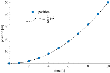
So, that’s the intro physics version. What happens when we try to make a computer simulation that captures this motion.

Here’s a quick sim that makes a ball move horizontally at a constant acceleration. The ball (an ellipse) follows the equation of motion presented above. The time variable increases by 1 every time the animation is redrawn. This works great!

var x=0, x0=0, v0=0, a=.05, t=0;
function setup() {
  createCanvas(600,100);
}

function draw() {
  background(100);
  t+=1;
  //equation of motion
  x = x0 + v0*t + 0.5* a * Math.pow(t,2);
  ellipse(x,height/2,10,10)
}

However, quickly we can see some limitations. What if the acceleration changes based on position. If, for example, we set the acceleration variable equal to zero when the ball moves halfway across the canvas, we would expect intuitively to keep going at a uniform velocity.

var x=0, x0=0, v0=0, a=.05, t=0;
function setup() {
  createCanvas(600,100);
}

function draw() {
  background(100);
  fill(120);
  rect(width/2,0,width/2,height);
  t+=1;
  //let's change the acceleration based on position
  if (x>width/2) {a=0;}
  //equation of motion
  x = x0 + v0*t + 0.5* a * Math.pow(t,2);
  fill(250);
  ellipse(x,height/2,10,10)

}

What happens is that when the particle reaches the halfway point – it’s position is set to zero. That makes sense now considering the equation of motion above. If $a$ and $v_0$ and $x_0$ are zero, the $x(t)$ will be zero too. Changing the acceleration using this method isn’t going to work because we would need to reset time to zero and change the initial positions and velocity.

So, instead of this equation of motion approach, the simulation of moving objects usually relies on an iterative approach: every frame, simply add some quantity to the previous frames position value. Like this:

var x=0, dx;
function setup() {
  createCanvas(600,100);
  dx = 1;
}

function draw() {
  background(100);
  x += dx;
  ellipse(x,height/2,10,10);
}

Now we can easily add an if() statement that changes the velocity of the particle at a certain point.

var x=0, vel;
function setup() {
  createCanvas(600,100);
  vel = 1;
}

function draw() {
  background(100);
  fill(120);
  rect(width/2,0,width/2,height);
  //if the particle goes past halfway, make the velocity 3 times faster.
  if (x>width/2){vel=3};
  x += vel;
  fill(255);
  ellipse(x,height/2,10,10);
}

That’s great. We have a particle whose speed we can control. What if we want to create an accelerating object? All we need to do is change the speed every frame also. One method for this that is commonly adopted is the following:

x = x + vel
vel = vel + accel

This psuedo-code says: take the position x and add the vel quantity. Also, add the accel quantity to the vel every frame too. This increases the velocity by a constant amount every frame, which then increases the position also.

Here’s a sim that shows it in action.

var x=0, vel, accel;
function setup() {
  createCanvas(600,100);
  vel = 0;
  accel = 0.05;
}

function draw() {
  background(100);
  x += vel;
  vel += accel;
  ellipse(x,height/2,10,10);
}

We can see it looks pretty good. The little ball is clearly accelerating across the screen.

Here’s a sim that has two balls. The green ball uses the kinematic equation from earlier, while the red ball uses this new iterative formulation.

var x0=0, x1=0, v0=0, a=.05, t=0, vel, accel;
function setup() {
  createCanvas(600,100);
  vel = 0;
  accel = .05;
}

function draw() {
  background(200);
  //method 1
  x = x0 + v0*t + 0.5* a * Math.pow(t,2);
  t+=1;
  fill('green');
  ellipse(x,height/1.5,10,10);
  //method 2
  x1 += vel;
  vel += accel;
  fill('red');
  ellipse(x1,height/2.5,10,10);
}

At first glance, everything seems cool. The two balls accelerate across the canvas at about the same rate. However, we can slow down the motion and take a closer look. We’ll reduce the frameRate() to 2 frames per second, crank up the acceleration to 11, and keep each ball’s position on the screen so we can track their progress.

var x0=0, x1=0, v0=0, a=11, t=0, vel, accel;
function setup() {
  createCanvas(600,100);
  vel = 0;
  accel = 11;
  frameRate(2);
}

function draw() {
  //method 1
  x = x0 + v0*t + 0.5* a * Math.pow(t,2);
  t+=1;
  fill('green');
  ellipse(x,height/1.5,10,10);
  //method 2
  x1 += vel;
  vel += accel;
  fill('red');
  ellipse(x1,height/2.5,10,10);
}

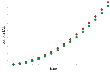
Now we see some discrepancies. The two particles are not aligned anymore. The red particle has jumped ahead from the get go, and continues to beat the green the particle across the canvas. If we look at the plots of the positions of these particles, we also see the same discrepancy - the red ball is covering more ground in the same amount of time.

How do we resolve this. Both object seem to be accelerating. Both have the same acceleration value, yet they move at different rates. So, maybe the red is just accelerating faster - that’s why. So, let’s fit the red curve to a quadratic function.

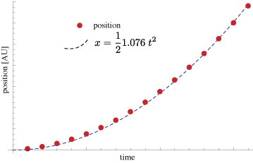
Here’s the result. Now, the trained eye will see a problem here. First, the acceleration is not quite equal to 1. And, what’s somehow more concerning, the dotted line, our quadratic, doesn’t line up the with red dots. Sure, the fit is close but, it’s not perfectly right. It’s as if this particle is not following the laws of motion precisely. Further analysis of these points indicate that the exponent of the polynomial that would fit to these red dots is a bit bigger than 2. So, our equation of motion might be more like:

\[x(t) = x_0 + v_0t + \frac{1}{2} a t^{2.03}\]

It’s not a big difference. Heck, we couldn’t even notice it by looking at the first example that compared the two particles above. But, it really should be 2. This is a computer simulation. There’s no friction, no wind, no air resistance, no nothing to make us deviate from our pure physical abstract land. Every thing should work out perfectly. Absolutely perfectly.

Fortunately, we have a solution. Check it out in Part 2.