Instructions:
Move the sliders to adjust the drag coefficients and launch angle. Press Save to store the last trajectory to compare.
Explanation:
This simulation plot the trajectory for a projectile that experiences a velocity dependant drag force. There are generally two type of drag forces: Stokes drag (depends linearly on the objects velocity), and Newtonian drag (depends on the velocity squared). Unlike projectile trajectories in vacuum, there are no analytically derivable solutions for the motion in general, so we must use numerical methods to calculate the trajectories, given a certain set of initial conditions.
$$ m \ddot{\mathbf{r}} = - m \mathbf{g} - b v \hat{\bf{v}} -c v^2 \; \hat{\bf{v}} $$
Or, if we separate the equation into component form.
$$ \begin{align} m \dot{v}_x & = - b v_x -c \sqrt{v_x^2 + v_y^2} \; v_x \\ m \dot{v}_y & = -mg -bv_y - c \sqrt{v_x^2 + v_y^2} \; v_y \end{align} $$
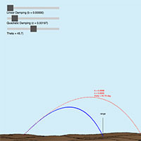
While no analytic solution is available for $x$ and $y$, we can use computational means to solve them. We'll use the Runge-Kutta 4th order approximation to create a trajectory for the projectile. In the simulation you can notice how some interesting physics developes. For example, the maximum range is no longer obtained when aiming with a $\theta$ of 45°.
Link to stand-alone sim: Here is a link to view the sim on its own, with no distractions.